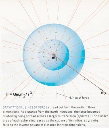
If one of the objects is much heavier than the other, e.g., m1 >> m2 like the Sun / Earth system, then m1 can be placed in the origin of the coordinate system and Eq.(1) can be solved as a one-body problem. In case the two masses are similar, the problem can be reduced to a one-body problem with a fictitious object moving around the center of mass, and Eq.(1) is still applicable. The equation of motion becomes rapidly un-manageable for system of three bodies and beyond. Eq.(1) would include accelerations for all the objects and the force on one object would involve the interaction with all the others. This is the situation often encountered in celestial mechanics with spacecraft flying among planets. The
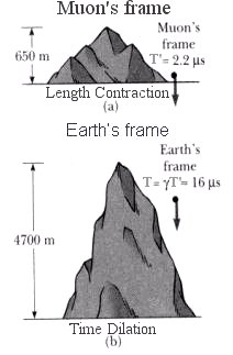
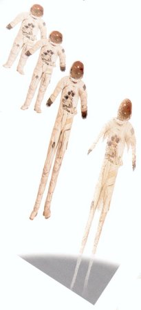
 = (1 - V2/c2)-1/2), show the muon decay as experienced in its own frame and from the view point of a stationary observer on Earth. The
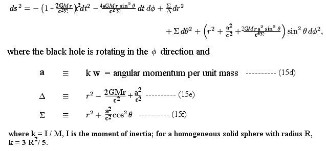
 G/c4) (Tik - gikT) ---------- (12a)
 ikl (dxk/ds) (dxl/ds) = 0 ---------- (12b)
 = 6
= 6 d
d 2 + d
2 + d , the space-time metric reduces to the expression for flat space-time:
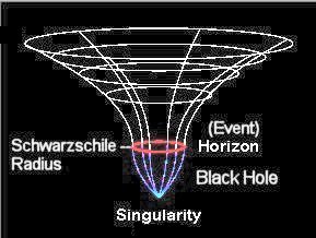
 =
= 
 2GM / rs3 =
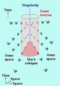
 to be the time associated with the moving frame, in which the spatial variation vanishes (co-moving objects are stationary in that frame), then
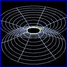
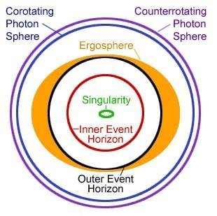
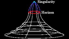
 , a singularity develops in the form of a ring at the equator (see Figure 09p), where
  g11 = cos2
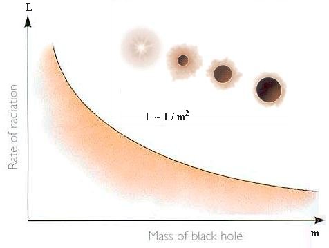
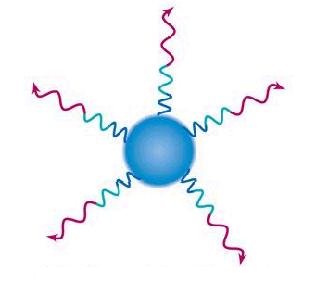
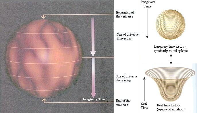
 ) x A, then T ~ 1 / m, and the rate of radiation L can be expressed as L ~ rs2T4 ~ 1 / m2. Therefore, as the black hole loses mass, its temperature and rate of emission increase, then it lose mass even more quickly (Figure 09r). What happens when the mass of the black hole eventually becomes extremely small is not quite clear, but the most reasonable guess is that it would disappear completely in a tremendous final burst of emission.
 , the gravitational field equation becomes:
 - 1) ---------- (18b)
 R2 c2 / 3 ---------- (20)
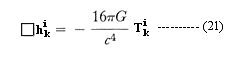
 is the d'Alembertian operator in four-

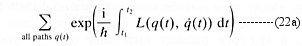
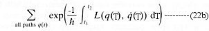
 = 0 ---------- (23)
