 |
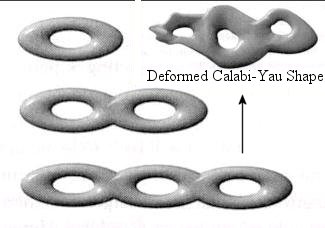
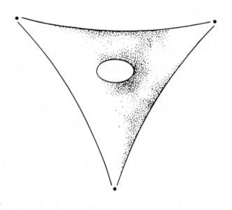
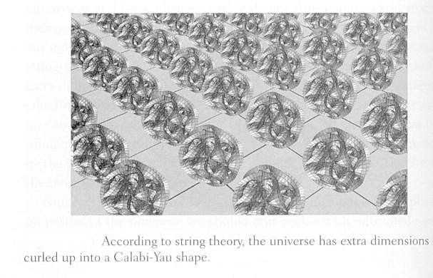
a family of lowest-energy string vibrations associated with each hole in the Calabi-Yau portion of space. Because the familiar elementary particles should correspond to the lowest-energy oscillatory patterns, the existence of multiple holes means that the patterns of string vibrations will fall into multiple families. If the curled-up Calabi-Yau has three holes, then we will find three families of elementary particles as observed. Unfortunately, the number of holes in each of the tens of thousands of known Calabi-Yau shapes spans a wide range from 3, 4, 5, 25, ... 480. |
 (
( ,
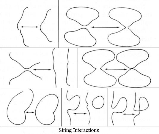
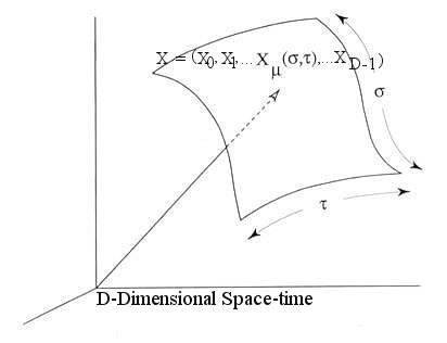
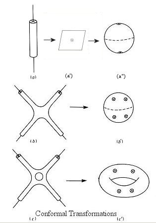
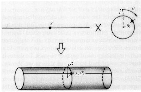
, ) trace out a curve as
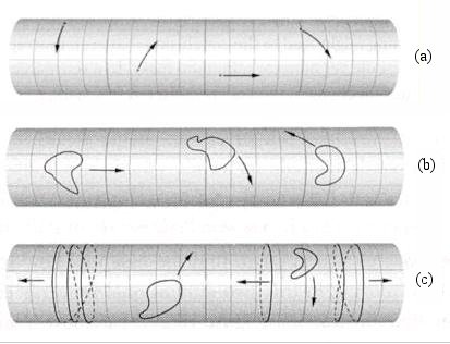
  as the string is traced out from on end to the other for an open string, or once round the string for a closed string. The string sweeps out a world sheet as
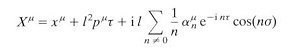
  = 1, c = 1):
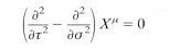
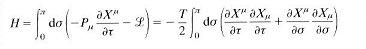
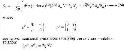
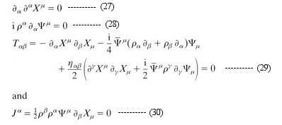
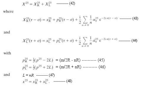
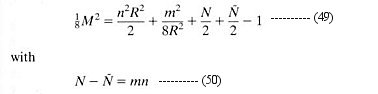
 to minimize the action, more equations can be derived in the form:
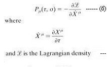
 may be interpreted as the energy-momentum tensor for a two-dimensional field theory of "D" free scalar field X
 n
n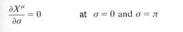

 ---------- (20)

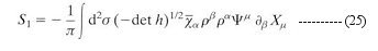
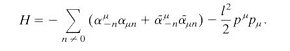
 This cancellation scheme in turn gives another extra term, which is finally cancelled by S2 -
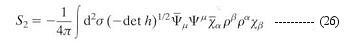


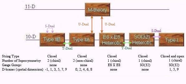
 called dilaton. It can be shown that the Type IIB theory is invariant under a global transformation by the group SL(2,R) with the dilaton field transforming as