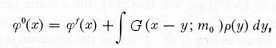
| ---------- (1) |
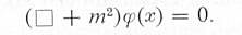
 is the field, which is a complex function (with real and imaginary parts) of x, y, z, and t (simply represented by x in the equation),
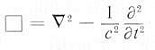 , and
, and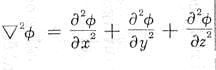
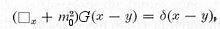
 | ---------- (2) |
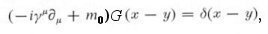
 | ---------- (3) |
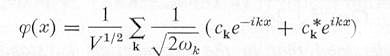
 , and the time x0 is set to zero after the time derivation has been performed.
 | ---------- (4) |
 | ---------- (5) |
 | ---------- (6) |
 | ---------- (7) |
 | ---------- (8) |
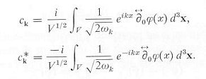
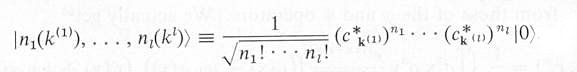
 | ---------- (9a) |
 | ---------- (9b) |

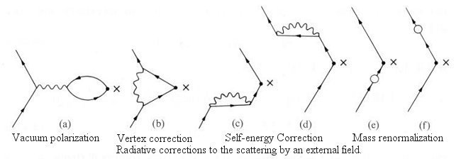
 is the Dirac matrices to keep track of the ferminon's spin.
  in general; it is equal to 1 for free field and 0 for a point source. The renormalized field, mass, and energy are
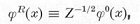
 and EnR = Z-1Eno respectively. The physical mass mR is the experimentally observed mass, mo is an unspecified parameter (called "bare mass") which together with Z-1 determine a value in agreement with experiment. In a realistic, fully quantized system, perturbation theory must be used to obtain any numerical result. However, it is found that perturbation theory calculations always lead to an infinity value for Z so that the "bare" quantities such as mo would also be infinity to yield a finite value for mR.
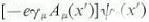 , where A is the electromagnetic vector potential and
  is the field for the fermion, which now appears on both sides in Eq.(8) (with
  (y) replaced by the interaction term,
  replacing
  , and K defined by Eq.(9b)). An iteration procedure yields a sum of integrals as shown in the formula below:
 |
---------- (10) |
0 in the first term is the free field solution, and the integration is over all the space-time x', x'', x''', ... Note that each of the following term is multiplied by the power of e, from e1, to e2, ... Since e=1/137 for the electromagnetic interaction, computation on a few terms would be sufficient to obtain a result with acceptable accuracy.  |
---------- (11) |
 |
---------- (12) ---------- (13) |
 | ---------- (14) |
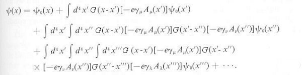
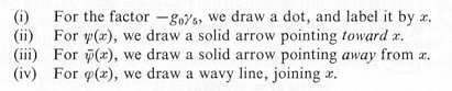
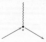
 the nth order term in the S-matrix expansion Eq.(11) has the explicit form:
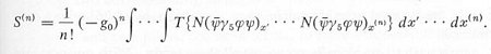 | ---------- (15) |
 | ---------- (16) |
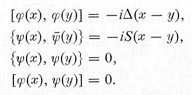
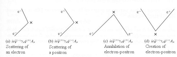
 . This is usually referred to as propagator and graphically represented by a wavy line running from x to y as show below:
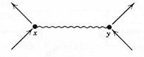
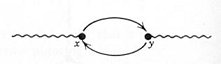
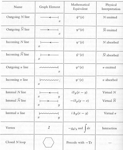
 represents the anti-nucleon. The subscript F in the propagator indicates that it satisfies causality.

 | ---------- (24) |
 | ---------- (36) |
 | ---------- (37) |


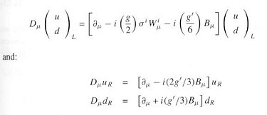
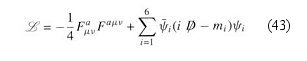
 Standard Model for the Standard Model. The field equations are derived by minimizing the action, which is related to the Lagrangian density. Thus instead of writing down the field equations explicitly such as in Eqs.(17) - (20) or Eqs.(13) and (38), the dynamics of the electro-weak interaction can be expressed in term of the Lagrangian density:
  in Eq.(40) consists of three parts. 1 is the gauge bosons part; 2 is the fermionic part; and 3 is the scalar Higgs sector, which generates mass for the gauge bosons and the fermions.
:
and
in Eq.(40) consists of three parts. 1 is the gauge bosons part; 2 is the fermionic part; and 3 is the scalar Higgs sector, which generates mass for the gauge bosons and the fermions.
:
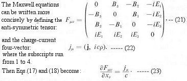
and  are indices for the space-time components running from 1 to 4. Whenever an index appears in both the subscript and superscript, it signifies a summation over these components. is related to the three gauge (vector) bosons with the index "a" running from 1 to 3. is the anti-symmetric tensor for the electromagnetic field as shown in Eq.(24), where the vector potential A is now denoted by B.
 | ---------- (42f) |
. are the Pauli matrices as shown in Eq.(10) in the appendix on "Groups" with i running from 1 to 3. The four 4X4
  metrices are constructed from the Pauli matrices and the identity matrix.
 is the scalar Higgs field as depicted in the diagram below:
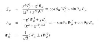
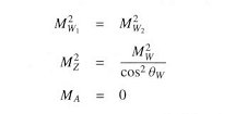
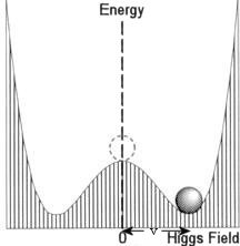 ' = - v, the fields Wa and B recombine and reemerge as the physical photon field , a neutral massive vector particle Z, and a charged doubled of massive vector particles W
 :
:
 = 0) to the more stable "true vacuum" (where = v). Gravitationally, it is similar to the more familiar case of moving from the hilltop to the valley. In the case of Higgs field, the transformation is accompanied with a "phase change", which endows mass to some of the particles.
 is similar to the SU(2) gauge field in Eq.(42a). This is essentially the Yang-Mills field developed back in 1953 by generalizing the gauge invariance used in QED. It represents the eight massless gluons carrying the SU(3) "colour" force with the index "a" running from 1 to 8.
  =
=  .
.