Chaos Theory

Contents

Non-linear Equations

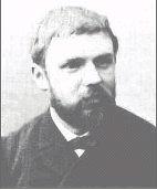
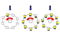
At the end of the 19th century, the French mathematician Henri Poincare tried to solve the differential equations for the three body problem. It was noticed that the orbit is not periodical anymore (in contrary to the case with just two body), actually the motion appears to be random. Then it was found that the solution is "exquisite sensitivity to initial conditions". The object would follow a very different path at the slightest change of initial condition. Figure 01 is an animation showing two paths of a third body under the gravitational influence of two massive objects. The paths start at the same position but the velocities differ by 1%. Initially the paths are very close, the difference becomes apparent after a while. Sixty years later, this kind of divergent behavior was re-visited by a meteorologist, named Edward Lorenz, with a set of 12 equations used to model the weather. He found the system evolves differently by just a very

Figure 01 Chaos [view large image]

slight variation of the initial condition. This divergent behavior is now known as the butterfly effect - the slightest disturbance of the air by a butterfly would cause a global weather change a year later. Eventually, Lorenz simplified the number of equations to three, and the system still

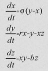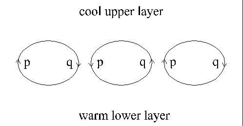
		exhibits the same kind of divergent behavior. The simplified system simulates the dynamical behavior of convection rolls in fluid layers that are heated from below (see Figure 02). This is a crude approximation of the air circulation at different latitude of the Earth (see Figure 09-10) It is also applicable to a leaky waterwheel. A waterwheel built from cups with equal sized holes in the bottom of each cup is allowed to turn freely under the force of a steady stream of water poured into the top cup. Figure 03 shows the Lorenz equations,
Figure 02 Lorenz System [view large image]	Figure 03 Lorenz Eqs.

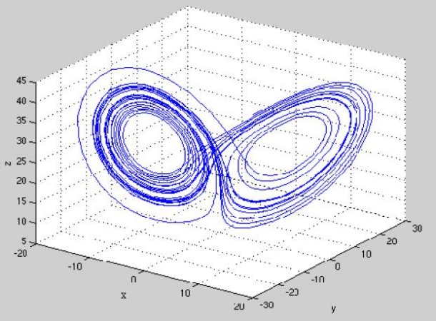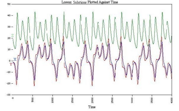
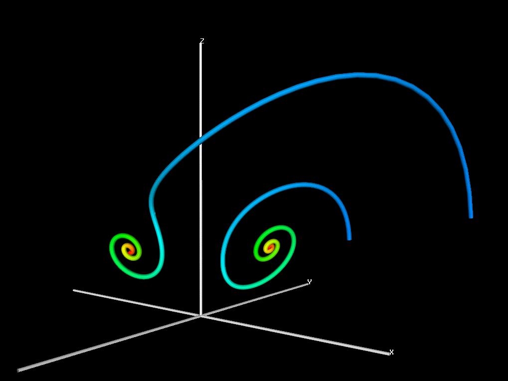
		development of the system is plotted in the phase space, where the values of x, y, z define each point in the graph. It is then clear that the system is confined to a certain region, namely the two shells (see Figure 05). However, the time progression of the points is not obvious. It either relies on color codes (for example, blue for earlier and red for later moment) or animation (which shows the points spreading from a small initial region) to display the evolution of the
Figure 04 Time Series [view large image]	Figure 05 Phase Space [view large image]	system. The region occupied by the system in the phase state, namely the butterfly or the shells, is known as Lorenz attractor, to which the dynamical motion will always converge no matter how far off initially.

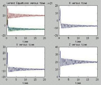
			The solutions of the Lorenz equations also depend on the parameters. When r is small, e.g., r = 10 all solutions tend to a fixed point. This is not chaos (see Figure 06). Starting from r ~ 14 the fixed points lose their stability. For r = 21, the system begins to exhibit transient chaos. This means that although it begins as a chaotic process, its long-
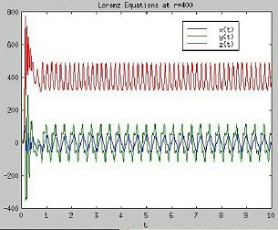
Figure 06 r = 10 [view large image]	Figure 07 r = 21 [view large image]	Figure 08 r = 400 [view large image]	term behavior becomes periodic (see Figure 07). The critical value for r that is required to produce chaos is r > 24. However, for very large value of r such as r = 400, all solutions become periodical again (see Figure 08).

Bifurcation

It turns out that the behavior of the solution depends on the growth rate R:


• For 0 < R < 1, the population will go extinct because there are fewer critters in each successive year.
• For 1 < R < 3, the population will survive and home in to a certain population level, X - a certain fraction of 1, the exact value depending on the value of R.
• For 3 < R, the population will also survive. But first it produces two alternating population sizes, each causing the other the following year. Here, the rhythm has shifted from a steady state to an alternating pattern. Increasing the value of R further will introduce a four repeating pattern. The next even smaller change will cause eight, then sixteen, then thirty two repeating cycles, ... The period doublings come faster and faster, until we have passed infinitely many of them. Still for a finite R, but the behavior becomes "chaos".
• For R = 4, whenever the value of X reaches 1 - the maximum, it inevitably follows by extinction as shown in Figure 09.
• For R > 4, values of X > 1 can be generated, and therefore negative X in the following year, i.e. the equation becomes unphysical (unbiological) beyond this point.

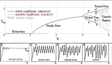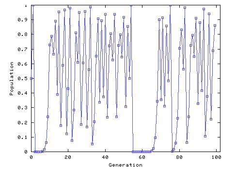
		Figure 10 is the graphic representation of the solutions. The lower diagrams are the time series for different value of R. The steady state reaches a stable value at Xm. The "period two" diagram shows two stationary points a and b, which are the maximum and minimum of the oscillation respectively. The "period four" diagram shows four stationary points c, d, e, and f. It looks like white
Figure 09 Logistic Eq. [view large image]	Figure 10 Bifurcation [view large image]	noise in the "chaos" diagram. Actually, there are so many stationary points, it is very difficult to follow the details. The upper diagram in Figure 10 plots the stable or stationary point Xm as a

Fractal

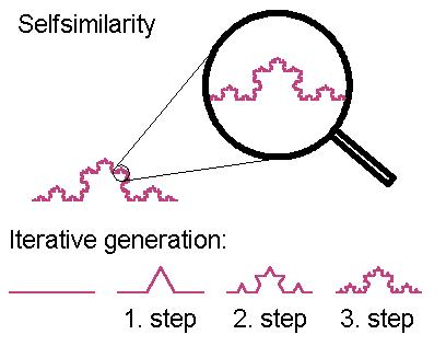The Koch curve has been constructed according to the idea of self-similarity. It starts from a straight line. Then add an equilateral triangle to the middle third of each side. A Kock curve is obtained by repeating the procedure on each successive (and shorter) straight line (see Figure 10). It is noticed the area enclosed within does not increase with the length of the lines as prescribed by the Euclidian geometry. To get around this difficulty, mathematicians invented fractal (fractional) dimensions. The fractal dimension of the Kock curve is somewhere around 1.26. Now fractal has come to mean any image that displays the attribute of self-similarity.

Figure 10 Koch Curve [view large image]

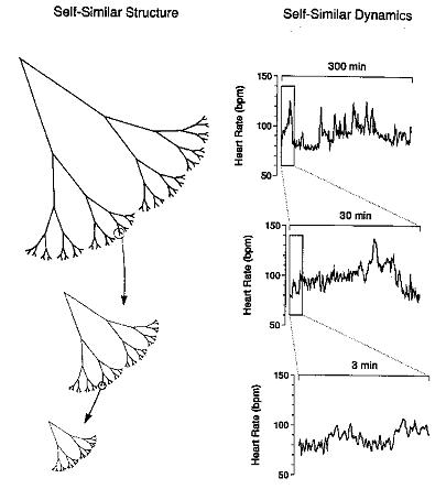
Figure 11 Fractal in Real-World [view large image]