Thermodynamics


Contents

Terminology
Systems
States
The Four Laws of Thermodynamics
Thermodynamic Process
Work and Engines
Connection to the Microscopic View

Terminology

Thermodynamics is the branch of science that deals with the conversions of various forms of energy and the effect on the state of a system. It was developed in the 19th century, when it was of great practical importance in the era of steam engines. Since the microscopic structure of matter is not known at that time, it can only prescribe a macroscopic view. It remains valid and useful in the 21th century, but now we understand such macroscopic description is just the averaged behaviour of a large collection of microscopic constituents.

[Top]


Systems

A thermodynamic system is that part of the universe that is under consideration. A real or imaginary boundary separates the system from the rest of the universe, which is referred to as the environment. A useful classification of thermodynamic systems is based on the nature of the boundary and the flows of matter, energy and entropy through it.
    There are three kinds of system depending on the kinds of exchanges taking place between a system and its environment:

  1. Isolated System - It does not exchange heat, matter or work with their environment. An example of an isolated system would be an insulated container, such as an insulated gas cylinder. In reality, a system can never be absolutely isolated from its environment, because there is always at least some slight coupling, even if only via minimal gravitational attraction.
  2. Closed System - It exchanges energy (heat and work) but not matter with the environment. A greenhouse is an example of a closed system exchanging heat but not work with its environment.
  3. Open System - It exchanges energy (heat and work) and matter with the environment. A boundary allowing matter exchange is called permeable. The ocean would be an example of an open system.

[Top]


States

A key concept in thermodynamics is the state of a system. A state consists of all the information needed to completely describe a system at an instant of time. When a system is at equilibrium under a given set of conditions, it is said to be in a definite state. For a given thermodynamic state, many of the system's properties (such as T, p, and ) have a specific value corresponding to that state. The values of these properties are a function of the state of the system. The number of properties that must be specified to describe the state of a given system (the number of degree of freedom) is given by Gibbs phase rule:

F = c - p + 2 ---------- (5)

where F is the number of degrees of freedom, c is the number of components in the system, and p is the number of phases in the system. Components denote the different kind of species in the system. Phase means a system with uniform chemical composition and physical properties.

For example, the phase rule indicates that a single component system (c = 1) with only one phase (p = 1), such as liquid water, has 2 degrees of freedom (F = 1 - 1 + 2 = 2). For this case the degrees of freedom correspond to temperature and pressure, indicating that the system can exist in equilibrium for any arbitrary combination of temperature and pressure. However, if we allow the formation of a gas phase (then p = 2), there is only 1 degree of freedom. This means that at a given temperature, water in the gas phase will evaporate or condense until the corresponding equilibrium water vapor pressure is reached. It is no longer possible to arbitrarily fix both the temperature and the pressure, since the system will tend to move toward the equilibrium vapor pressure. For a single component with three phases (p = 3 -- gas, liquid, and solid) there are no degrees of freedom. Such a system is only possible at the temperature and pressure corresponding to the Triple point.

One of the main goals of Thermodynamics is to understand these relationships between the various state properties of a system. Equations of state are examples of some of these relationships. The ideal gas law,

p V = n R T ---------- (6)

is one of the simplest equations of state. Although reasonably accurate for gases at low pressures and high temperatures, it becomes increasingly inaccurate away from these ideal conditions. The ideal gas law can be derived by assuming that a gas is composed of a large number of small molecules, with no attractive or repulsive forces. In reality gas molecules do interact with attractive and repulsive forces. In fact it is these forces that result in the formation of liquids.

[Top]


The Four Laws of Thermodynamics

[Top]


Thermodynamic Process

Thermodynamic process is a way of changing one or more of the properties in a system resulting in a change of the state of the system. The following summarizes some of the more common processes:

[Top]


Work and Engines

The dominating feature of an industrial society is its ability to utilize sources of energy other than the muscles of men or animals. Most energy supplies are in the form of fuels such as coal or oil, where the energy is stored as internal energy. The process of combustion releases the internal erergy and converts it to heat. In this form the energy may be utilized for heating, cooking, ... etc. But to operate a machine, or to propel a vehicle or a projectile, the heat must be converted to mechanical energy, and one of the problems of mechanical engineer is to carry out this conversion with the maximum possible efficiency.

The energy transformations in a heat engine are conveniently represented schematically by the flow diagram in Figure 01. The engine itself is represented by the circle. The heat Q2 supplied to the engine is proportional to the cross section of the incoming "pipeline" at the top of the diagram. The cross section of the outgoing pipeline at the bottom is proportional to that portion of the heat, Q1, which is rejected as heat in the exhaust. The branch line to the right represents that portion of the heat supplied, which the engine converts to mechanical work. The thermal efficiency Eff(%) is expressed by the formula:

Eff(%) = W / Q2 = (Q2 - Q1) / Q2 ---------- (6)

heat Flow Carnot Cycle The most efficient heat engine cycle is the Carnot cycle, consisting of two isothermal processes and two adiabatic processes (see Figure 02). The Carnot cycle can be thought of as the most efficient heat engine cycle allowed by physical laws. When the second law of thermodynamics states that not all the supplied heat in a heat engine can be used to do work, the Carnot efficiency sets the limiting value on the fraction of the heat which can be so used. In order to approach the Carnot efficiency, the processes involved in the heat engine cycle

Figure 01 Heat Engine [view large image]

Figure 02 Carnot Engine Cycle
[view large image]

must be reversible and involve no change in entropy. This means that the Carnot cycle is an idealization, since no real engine processes are reversible and all real physical processes involve some increase in entropy.
Gasoline Engine Diesel Engine Steam Engine The p-V diagrams for the more realistic cases are shown in Figure 03, 04, and 05 for the gasoline, diesel, and steam engines respectively. While the gasoline and diesel engines operate at about 50% efficiency, the steam engine runs at only about 30%. A brief description of the processes can be found in each of the diagram.

Figure 03 Gasoline Engine [view large image]

Figure 04 Diesel Engine [view large image]

Figure 05 Steam Engine [view large image]


[Top]


Connection to the Microscopic View

The branch of physics known as statistical mechanics attempts to related the macroscopic properties of an assembly of particles to the microscopic properties of the particles themselves. Statistical mechanics, as its name implies is not concerned with the actual motions or interactions of individual particles, but investigates instead their most probable behavior. The state of a system of particles is completely specified classically at a particular instant if the position r and velocity v of each of its constituent particles are known. The number of particles occupying an infinitesimal cell in the phase space r and v is determined by the distribution function f (r,v,t), where t is the time. The distribution function is normally conserved except from the effect of collisions. Thus, the most general formula for the evolution of the distribution function can be expressed as:

---------- (7)
where the pairing indices (in the subscript and superscript) indicate a sum over i = 1, 2, 3; ai is the acceleration related to the force on the particles, and the right-hand side of the equation represents the effect of collisions.

Boltzmann Equation This is known as the Boltzmann equation. It is very useful as mathematic tool in treating the process of fluid flow. By expanding the distribution funciton in terms of the power of the velocity - v0, v1, and v2, the equilibrium distribution in the form of Maxwell-Boltzmann distribution, the continuity equation, and the Navier-Stokes equations in fluid dynamics can be derived directly from Eq.(7). Analytical solutions of the Boltzmann equation are possible only under very restrictive assumptions. Direct numerical methods for computer simulation have been limited by the complexity of the equation, which in the complete 3-D time-dependent form requires seven independent variables for time, space and velocity. A 2-dimensional animation of a flow process is presented by clicking Figure 06. It shows the development of a clump of gas molecules initially

Figure 06 Boltzmann Equation Simulation [view animation]

released from the left. The particles flow to the right, reflected by the wall at the other end, then established an equilibrium configuration after some 4000 collisions between the particles.
Considering the simplest case when the force on the particles is switched off instantaneously. If the distribution is space-independent, then Eq.(7) is reduced to:
---------- (8)
The collision term on the right hand side of Eq.(7) is substituted by a phenomenological term in Eq.(8), where 
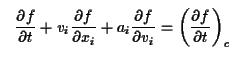
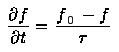
is the relaxation time - a characteristic decay constant for returning to the equilibrium state, and f0 is the equilibrium distribution. The solution for this equation is:

f = fi e-t/ + f0 ( 1 - e-t/ ) ---------- (9)

where fi is the initial distribution. It shows that f approaches f0, and the collision term vanishes for time t >> .

In thermodynamic equilibrium the distribution function f 0 does not change with time, it can be expressed in the form:

---------- (10)
where the density and temperature can be a function of r in general, and v0 is the velocity of the gas moving as a whole.

In the special case when there are no external forces such as gravity or electrostatic interactions, the density and temperature are constant, and v0 = 0, Eq.(10) can be written as:

---------- (11)
which is called Maxwell-Boltzmann distribution, where N is the total number of particles. It is actually a formula about the distribution of kinetic energy E = mv2/2 among the particles.

There are three kinds of energy distribution function depending on whether the particles are treated as classical or quantum. In quantum theory, the wave packets overlapped when the particles come together, it is impossible to distinguish their identities. Thus, it results in different behaviour in quantum statistics. Further modification is caused by the exclusion principle, which allows only one fermion in a given state. Figure 07 shows the formula and graph for each distribution, where A = e 
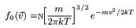
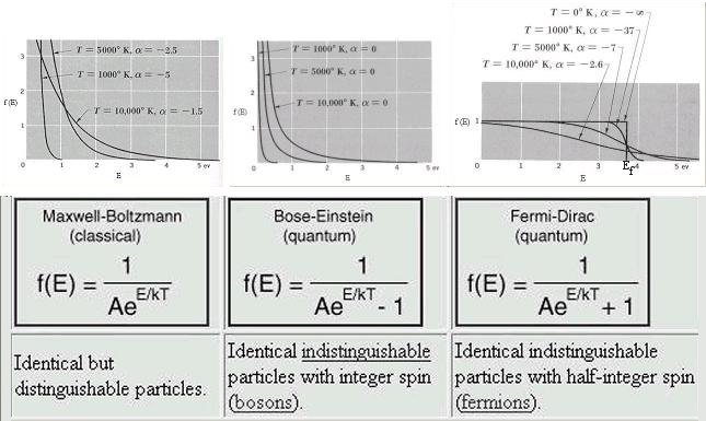
is a normalization constant. The classical and Bose-Einstein distribution are similar except when kT >> E. Near absolute zero
Distribution Functions temperature, most of the bosons occupy the same state with E ~ 0. This is the Bose-Einstein condensate first discovered in 1995. Another example of Bose-Einstein distribution is the black-body radiation. In Fermi-Dirac distribution, the normalization constant A can be re-defined as A = e-Ef, where Ef is known as the Fermi energy, which has a value of a few ev for the electron gas in many metals. Note that f (E) = 1/2 at E = Ef for all temperatures. At low temperature most of the low energy states with E < Ef are filled. At high temperature with kT >> (E - Ef),

Figure 07 Distribution Functions
[view large image]

the distribution function becomes f (E) ~ (1/2) (1 - (E - Ef) / 2kT). Thus in this case, the energy states with E < Ef are more than half-filler; while for E > Ef they are less than half-filled.
Maxwell Distribution In classical statistic, the velocity distribution of the ideal gas is given by the Maxwell distribution as shown in Figure 08. A relationship between the root-mean-square velocity vrms and the temperature T can be derived from such distribution function:

m vrms2 = 3 k T    or   M vrms2 = 3 R T ---------- (12)

where m denotes the mass of the molecule, M = mN0 is the molecular weight/mole, N0 is the Avogadro's number, and k = R / N0 = 1.38x10⁻¹⁶ erg/Ko is the Boltzmann constant .

Figure 08 Maxwell Distribution [view large image]

The formula in Eq.(12) provides a link between the microscopic root-mean-square velocity vrms of the particles and the macroscopic property T.

In order to determine whether to use thermodynamics (a macroscopic description) or statistical mechanics (with microscopic consideration), the Knudsen number K is evaluated for the problem. It is the ratio of the molecular mean free path length l to a representative physical length scale L, i.e., K = l / L . Problems with Knudsen numbers at or above unity, i.e., long mean free path; must be evaluated using statistical mechanics for reliable solutions. Dense system with K<1 can be treated as continuum.
Mean Free Path
The mean free path (Figure 09) can be expressed mathematically as:

l = 1 / nA = (l1 + l2 + l3 + ... + lN) / N---------- (13)

where n is the number density, A is the collision cross section, li is the path length between collisions, i.e., length of the free path, and N is the total number of collisions. The concept of mean free path may be visualized by thinking of a man shooting a rifle aimlessly into a forest. Most of the bullets will hit trees, but some bullets will travel much farther than others. The

Figure 09 Mean Free Path [view large image]

average distance traveled by the bullets will depend inversely on both the denseness of the woods and the size of the trees.