| Home Page | Overview | Site Map | Index | Appendix | Illustration | FAQ | About | Contact |
|
|
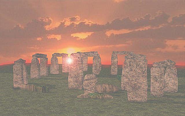
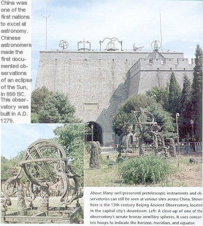
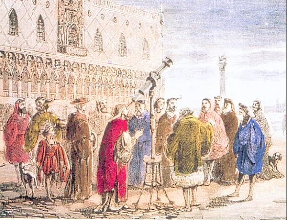
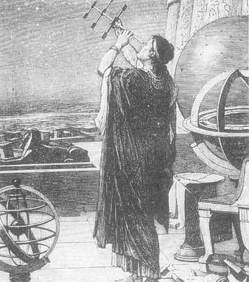
The Stonehenge (Figure 08-01a) is possibly the oldest astronomical instrument. It was built around 1500 BC outside Salisbury, England to track the movement of the sun and mark the solstice. The first record of a total eclipse of the sun was made in China as early as 899 BC. Figure 08-01b is the 13th-century Beijing Ancient Observatory - one of the most advanced facilities in the pretelescopic era. Modern astronomical instrument was first constructed by Galileo Galilei (1564-1642). He used a 30X |
Figure 08-01a Stonehenge |
Figure 08-01b Ancient Observatory [view large image] |
telescope from lenses made by himself to draw a picture of the moon. He also discovered sun spots and Jupiter's 4 satellites. More detailed description of the instruments used by astronomers today can be found in the appendix: Astronomical Instruments. |
 |
 |
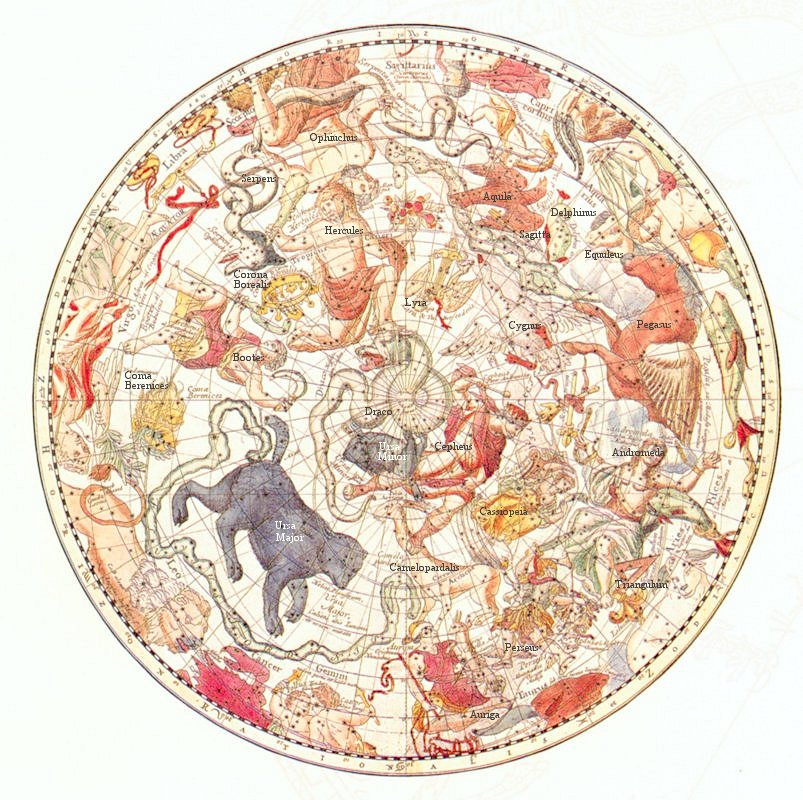
constellations are now used to locate the general direction of an object on the celestial sphere (see Figure 08-01e). To bring order from the chaos of naming stars, around the year 1600 Johannes Bayer, in what is now Germany, applied lower case Greek letter names to the stars more or less in order of brightness, rendering the brightest star in a constellation "Alpha", the second "Beta", and so on. To the Greek letter name is appended the Latin possessive form of the constellation name. Thus the brightest star in Orion is Alpha Orion, which is also known as Betelgeuse. |
Figure 08-01c Constalla- tions [view large image] |
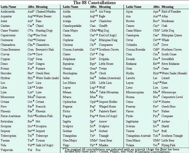
Figure 08-01d Constallation Names [view large image] |
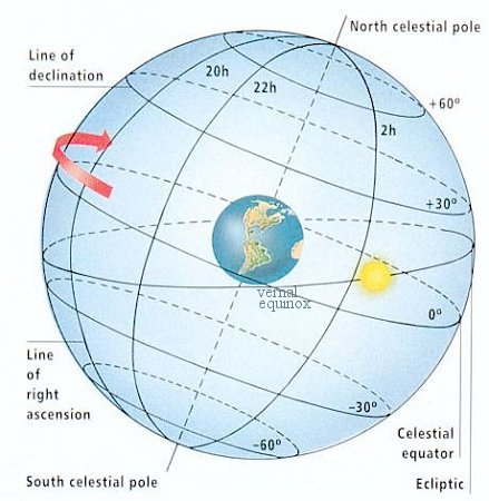 |
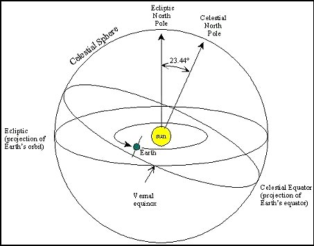
The positions of stars and other heavenly bodies are described by coordinate systems imposed onto an imaginary celestial sphere with the Earth (or the Sun) located at the center as shown in Figure 08-01e. The red arrow indicates the sphere's apparent daily movement westward (corresponding to the Earth's eastward rotation - counter-clockwise). There are 4 commonly used coordinate systems on the celestial sphere:
|
Figure 08-01e Celestial Sphere [view large image] |
south with a negative value and ends with -90o at the South Pole. This is the system most commonly used in astronomy. |
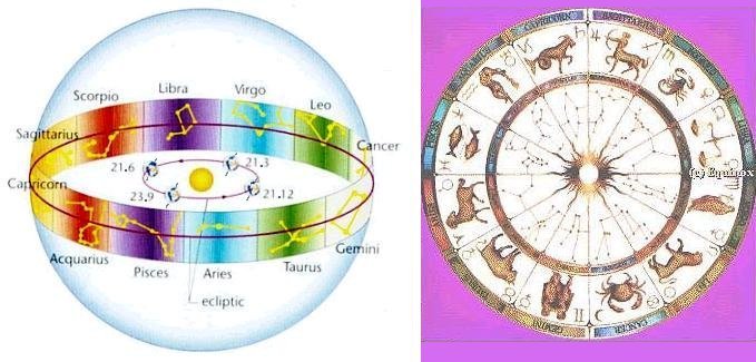 |
The Zodiac is a band of sky 18o wide across the ecliptic (Figure 08-01f): the ancients divided it from the gamma point (at the vernal equinoxe near Aries about 2000 year ago) into 12 signs 30o wide each, and to each sign gave the name of its most representative constellation. As the positions of the Earth and the other celestial bodies change, the Sun, the planets and the Moon are projected onto the Zodiac. During the year the Sun passes through all the signs as it moves |
Figure 08-01f Ecliptic and Zodiac [view large image] |
along the ecliptic. Each night we view a slightly different part of the Zodiac because of this revolution. The precession of the equinoxes has since moved the gamma point about 30o toward the constellation Pisces. |
 |
|
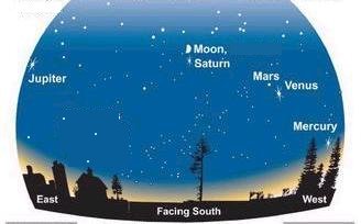
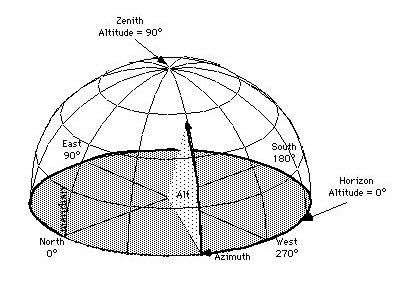
Figure 08-01g Horizon Co- ordinates [view large image] |
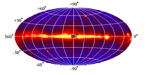 |
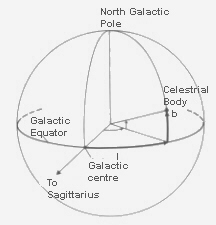
based on observations of the 21-centimeter line, a new system of galactic coordinates was adopted with the origin at the galactic center in Sagittarius at R.A. 17h 42.4m, Dec. -28� 55' (epoch 1950). The new system is designated by a superior Roman numeral II (i.e., bII, lII) and the old system by a superior Roman numeral I. Galactic coordinates are used to specify the position of objects in the Milky Way as observed from the Earth. |
Figure 08-01h Galactic Co- ordinates [view large image] |
The apparent magnitude m is a measure of the amount of light arriving on Earth from a star or other celestial objects. The brighter object has a smaller apparent magnitude. This curious property of "less is more" is a result of the work of Hipparchus (c130 BC) who classified stars into six magnitudes. The �first magnitude stars� were the brightest in the heavens, which included Capella (alpha Aurigae), Sirius (alpha Canis Majoris), Vega (alpha Lyrae) and the like. Hipparchus categorized the other stars according to their relative brightness, down to the dimmest that the naked eye could see, which were called sixth magnitude.
In simple mathematic the apparent magnitude is defined by the formula:
 |
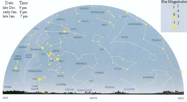 |
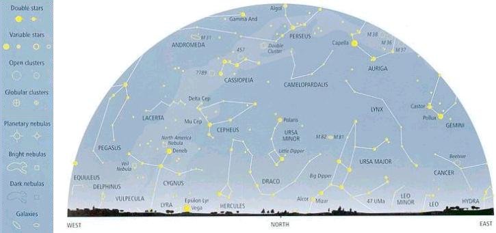
latitude 10 to 15 degrees north or south of this) - suitable for viewing in the United States, Canada, Europe, and Japan. The Southern Hemisphere charts usually depict the sky from a latitude of 35oS. These are for use in the South Pacific, Australia, New Zealand, South America, and southern Africa. |
Figure 08-01f Sky Chart, North [view large image] |
Figure 08-01g Sky Chart, South [view large image] |
 |
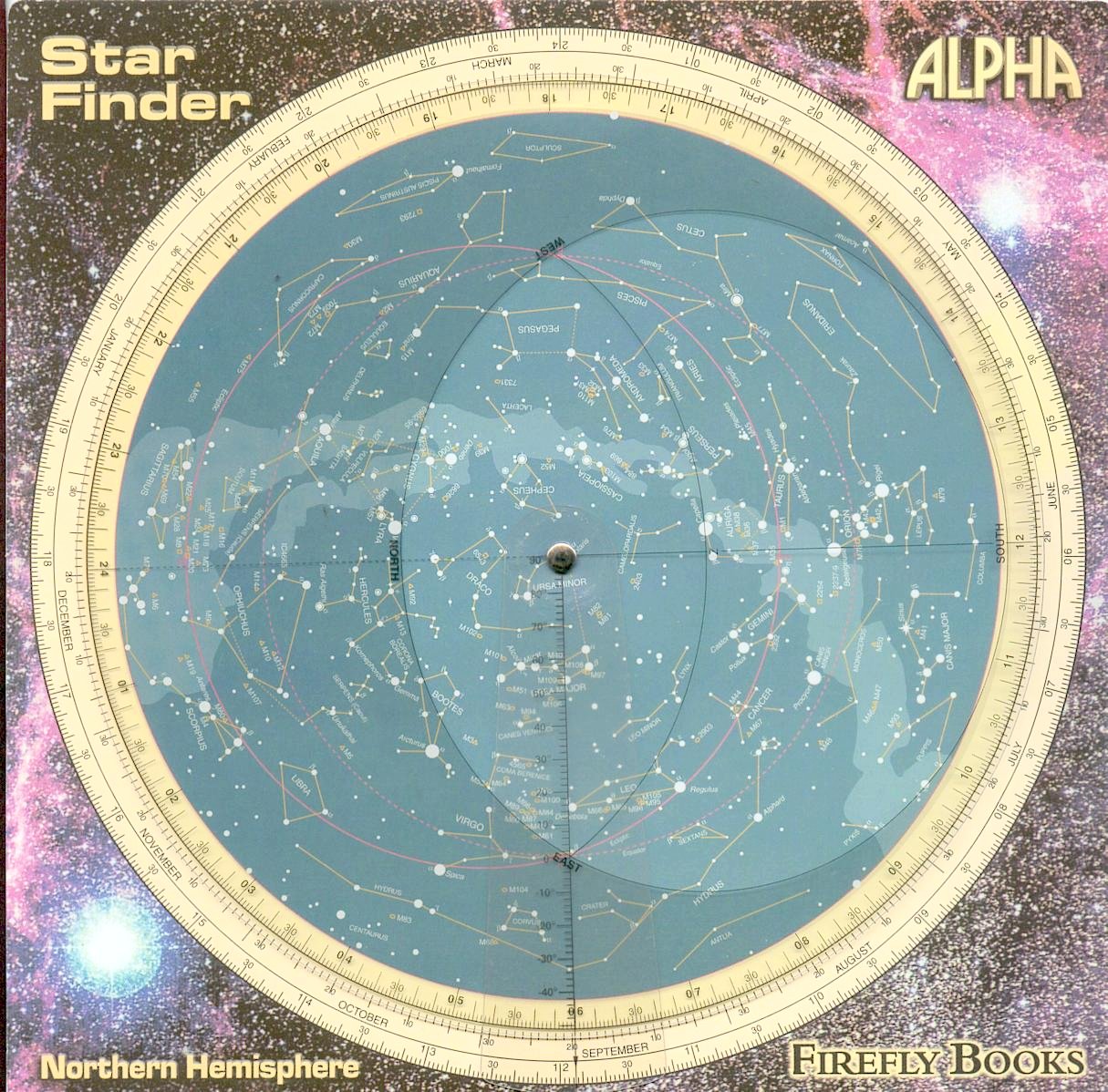 |
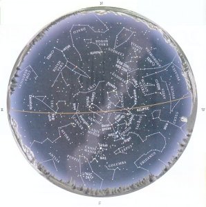
Figure 08-01h shows the entire Northern sky in late January. An one piece sky chart plots the sky with the North Pole at its center (see Figure 08-01i). An oval opening in an overlapping disc represents the heavens as seen from a certain latitude, e.g., 45oN. The time and date of viewing can be selected by rotating the disc around the center. This particular view is set at 22:00 h, January 20. The transparent cursor scale (from -50o to 90o) is used to calculate the declination of celestial objects. The right ascension is marked at the outer-most circle. |
Figure 08-01h Sky Chart [view large image] |
Figure 08-01i Star Finder [view large image] |
 |
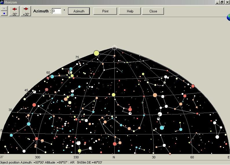 |
Sky charts computer software is perhaps the most versatile. It allows the user to specify any location and date/time as shown in Figure 08-01j, which displays a chart tailored to "Sample" with latitude 42o and longitude 270o at 22:00 h on January 20, 2004. The detail of objects can be adjusted by the user. It can display the ecliptic as well as the Galactic equator. The coordinate grids can be numbered. Outline of the Milky Way can be plotted on the chart. The name of each object (if not |
Figure 08-01j Sky Chart, Computer Generated |
Figure 08-01k Sky Chart, Horizon |
already shown) can be obtained by clicking the pointer (such as NGC2539 in the sample chart). Figure 08-01k shows the same chart in horizon coordinate facing North. This free sky charts software is offered by Cartes du Ciel. |
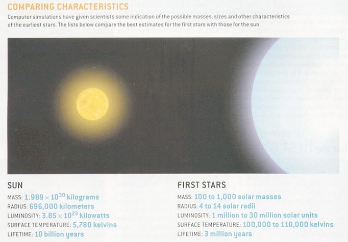 |
The first stars appeared about 100 million years after the Big Bang. It formed in the denser regions of gas inside the protogalaxies. The protogalaxies in turn would be most likely located at the nodes of the filaments in the large structure. Since there was little metals present in the early universe, the production of nuclear energy is less efficient, the first stars were able to assemble more mass and still maintained a stable structure. The limit should be no more than 1000 solar mass. Figure 08-02 compares the calculated characteristics of the first stars with those for the Sun. The most iron-deficient star HE0107-5240 was discovered in late 2002. This primitive star has a measured abundance of iron less than 1/200000 that of the Sun. It seems to have formed shortly after the Big Bang. |
Figure 08-02 First Stars [view large image] |
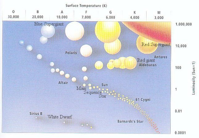
The Hertzspung-Russell diagram was introduced in the 1910s to plot a point representing a star with a certain values of luminosity and surface temperature as shown in Figure 08-03.
 |
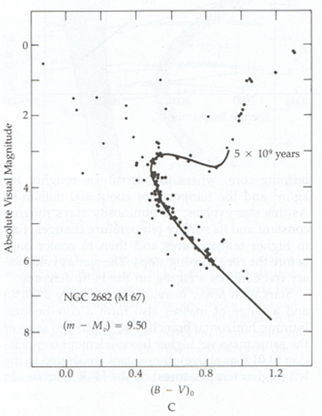
It soon became apparent that the HR diagram is not randomly populated, but that stars preferentially fall into certain regions. The majority of them occupy a strip called main sequence as depicted by the red line in Figure 08-03. This just reflects the fact that all the stars spend most of their time burning off hydrogen fuel with a constant luminosity and surface temperature. There are variable stars, which change their brightness, color, spectrum and other characteristics in the order of hours to few hundred days. They appear as a transient phenomenon in the HR diagram. The evolutionary track of an individual star with a given mass can be traced in the HR diagram as shown in Figure 08-04, 08-05, and 08-06. The age of the globular clusters can be estimated from the branch-off point in the HR diagram. The HR diagram comes with many variations since luminosity and temperature are related to other quantities. For example, in the vertical axis on the right of Figure 08-03, the label is Absolution Magnitude. Since different temperature of the stars generate different set of absorption lines, this scale can be translated into spectral types such as O, B, A, F G, K, and M as shown in the horizontal axis at the bottom of Figure 08-03. Each spectral type is further subdivided into numerals, e.g., G2 for the Sun, which is located in the middle of the main sequence. Sometimes the horizontal axis is labelled by the colour index B - V or mB - mV, i.e., magnitude in blue - magnitude in visual |
Figure 08-03 HR Diagram |
(yellow) with blue objects in the left and yellow objects to the right. It is a directly measurable quantity from photometer with colour filters. |
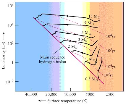 |
Figure 08-04 is another version of the HR diagram. It shows the progression of mass along the main sequence, and the pre-main-sequence evolutionary track for different masses from 0.5 to 15 Msun. The mass of a star determines all its properties in the HR diagram. The observed upper limit for stellar mass is about 60 Msun, the star becomes unstable beyond this limit. The heavy star will be an O type located at the upper left corner of the main sequence. The observed lower limit is about 0.05 Msun occupying a position down in the lower right corner of the main sequence as M type stars. Protostar below this limit is not able to ignite hydrogen burning and becomes a brown dwarf. The contraction time to the main sequence is plotted as contours in range from 104 to 107 years. The pre-main-sequence stars begin their life as interstellar clouds (with a size of several light years), which |
Figure 08-04 HR Pre-Main-Sequence [view large image] |
collapse under the influence of gravity to a stage called T Tauri stars before settling down onto the main sequence (see Figure 08-07). In tabulation form, Table 08-01 lists some characteristics of main-sequence stars as a function of mass. |
| Mass (Msun) | Spectral Type | Luminosity (Lsun) | Diameter (Dsun) | Central Density (Water=1) | Lifetime (109 yrs) |
|---|---|---|---|---|---|
| 0.1 | M7 | 0.0001 | 0.1 | 60 | 1000 |
| 0.5 | K8 | 0.03 | 0.7 | 80 | 100 |
| 1 | G2 | 1 | 1 | 90 | 10 |
| 1.5 | F3 | 5 | 1.3 | 85 | 1.8 |
| 2 | A6 | 17 | 1.7 | 70 | 0.8 |
| 5 | B8 | 500 | 3 | 20 | 0.075 |
| 10 | B5 | 5000 | 5 | 9 | 0.02 |
| 15 | B1 | 20000 | 10 | 6 | 0.01 |
| 30 | O8 | 100000 | 15 | 3 | 0.004 |
 |
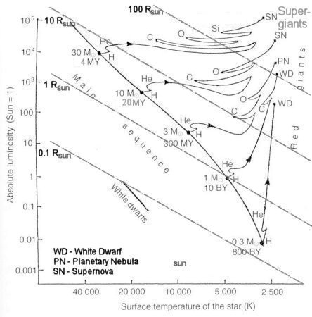 |
The structure of a star is maintained in equilibrium via the balance of the gravitational attraction with a tendency to contract and the thermal pressure with a tendency to expand. When the star has exhausted its hydrogen fuel, it cools off and collapses until the pressure has risen sufficiently to ignite helium and other types of nuclear burning. This process of re-igniting fuel burning with different nuclear species is represented by the zigzag paths in Figure 08-05b. The variation of stellar radius can be traced with the curves |
Figure 08-05a HR Post-Main-Sequence, Sun [view large image] | Figure 08-05b Post-Main-Sequence [view large image] |
crisscrossing the loci of constant radius. It shows that the maximum extent can be 100 Rsun or more and hence the names of giant, and supergiant. |
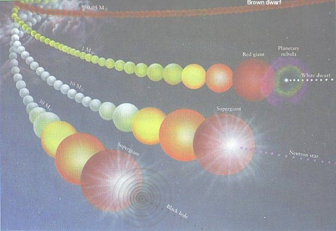 |
These stars have evolved to the terminal phase as shown in Figure 08-05a and 08-05b. Eventually, all the available fuels are consumed, there is no more source to supply the thermal pressure necessary to stop further collapsing. However, for star with mass smaller than 5 Msun the degeneracy pressure of the electrons lends its support to stop complete collapse and it forms a white dwarf with remnant less than 1.4 Msun. For star with mass in between 5 and 15 Msun the protons combine with electrons to form neutrons under the tremendous pressure. Then the degeneracy pressure of the neutrons can provide support up to 3 Msun (of the remnant) and it becomes a neutron star (or pulsar - spinning neutron |
Figure 08-06 Stellar Evolution |
star). For star with mass greater than 15 Msun, no amount of support is sufficient to stop the collapse to a black hole. Figure 08-05a portrays the post-main-sequence evolutionary track for the Sun in details. |
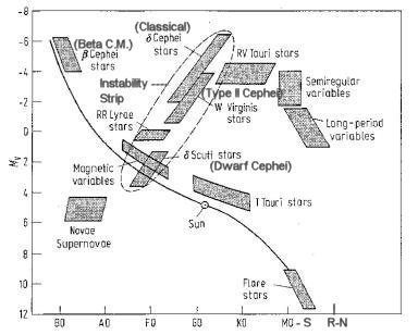 |
The changes of brightness in (intrinsic) variable stars indicate that something is happening to them. The cause must be truly physical, because changes of color, spectrum, magnetic field, and radial velocity accompany the changes in light. Some variable stars display a more or less regular rhythm, or period, and are known as the periodic variables. Others, only roughly periodic, are know as the cyclic or semiregular variables, and then there are stars whose variations show no obvious pattern, the irregular variables. Far more spectacular are the changes shown by some stars that undergo some sort of explosion - the so-called cataclysmic variables. These include the novae (new stars), and the |
Figure 08-07 HR, Variable Stars [view large image] |
supernovae, which undergo the largest changes and attain the greatest luminosities recorded for any variable or nonvariable stars. Figure 08-07 shows the various types of variable stars in the HR diagram. Table 08-02 summarizes the properties of all the types. |
| Type | Period Range | Mag. Range |
Spectral Types | Mean Abs. Mag. | Space Distribution |
|---|---|---|---|---|---|
| Classical Cepheids | 2 - 8 d | 1 | F, G superg. | -3 | Dust-filled galactic plane |
| RR Lyrae | 0.1 - 1 d | 1 | A, F giants | 0 | Dust-free galactic nucleus |
| Type II Cepheids (W Vir, RV Tau) |
1 - 100 d | 1 | F-G, G-K | -2 | High galactic latitude, halo |
| Long Period | 90 - 600 d | 3 - 6 | M,S,R,N (em) | -1, 0 | Dust-free galactic plane |
| Semiregular | ~ 100 d | 1 | M,S,R,N | -2 | Dust-filled galactic nucleus |
| Irregular | 0.1 | M,S,R,N | -2 | Dust-filled galactic nucleus | |
| Beta Cepheids (CM) | 3 - 6 h | 0.1 | B | -3 | Dust-Filled regions |
| Dwarf Cepheids | 1 - 3 h | 0.2 - 1 | A - F | +2 | Dust-filled regions |
| Magnetic or Spectrum | 0.5 - 1 d | 0.1 | A | 0 | |
| R Coronae Borealis Stars | irrg. (fading) | 6 | G, K, R (em) | -3 | Low galactic lat., carbon stars |
| Flare Stars | irrg. | 6 | K, M (em) | +10 | Lower main sequence stars |
| T Tauri Stars | irrg. | 1 - 3 | G, K - M | +5, +2 | Dark clouds of dust & gas |
 |
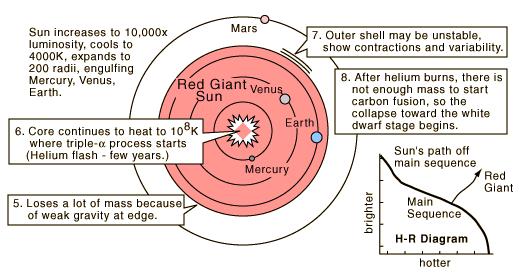 |
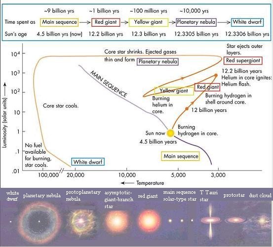
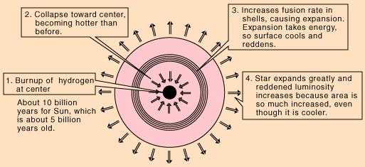
high and the total luminosity is also high. Since the average luminosity is low, the star appears red. This big red star is a red giant. Figure 08-08a is a schematic diagram depicting this initial phase of a red giant with a (main-sequence) mass of 1 Msun. |
Figure 08-08a Red Giant 1 |
Figure 08-08b Red Giant 2 [view large image] |
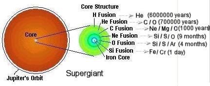 |
an even larger volume. The much brighter, but still reddened star is called a red supergiant (it is blue supergiants for O, B stars). Some of these supergiants are unstable and form the very important Cepheid variables (as standard candles for determining distance to galaxies). In their final stages, supergiants will explode into supernovae. The collapse of these massive stars may produce a neutron star or a black hole. |
Figure 08-09 Supergiant |
 |
 |
 |
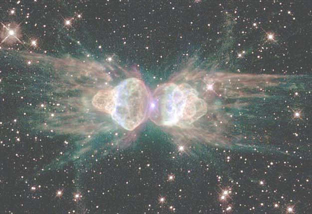
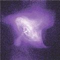
When a star with mass less than 5 Msun reaches the end of its life, it casts off its gaseous outer-envelope at high speed (1000-2000 km/sec) and leaves behind a planetary nebula as shown in Figure 08-10 (click on image to obtain larger view). The one on the left is the side view in bipolar appearance, while the Helix Nebula in |
Figure 08-10 |
Planetary Nebulae |
the middle is the end-on view. The right image shows ten different planetary nebulae in a |
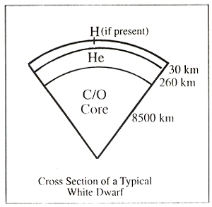 |
The shrinking core of a low mass star cannot contract far enough to raise its temperature high enough for carbon burning to commence. No further thermonuclear energy generation is possible. The shrunken remnant becomes a white dwarf with a size comparable to the Earth and is composed predominantly of carbon and oxygen. The structure is supported by electron degeneracy pressure. The matter in the white dwarf is packed very tight (up to 3x10⁷ gm/cm3 in the core) in layers (see Figure 08-11). Under such conditions of high density the atomic electrons are no longer attached to individual nuclei. The electrons are ionized and form an electron gas. In the absence of nuclear energy sources, the star cools down, but, because degeneracy pressure is unaffected by the decreasing temperature, the cooling white dwarf does not contract. It instead continues to cool and to fade away gradually. Over ten billions years or more it will |
Figure 08-11 White Dwarf [view large image] |
eventually evolve to become a cold dark body called a black dwarf. This process takes so long that there has not been enough time since the origin of the universe for any star to reach the black dwarf state. Table 08-03 compares the properties of the Sun, the Earth, and Sirius B - a typical white dwarf. |
| Property | Sun | Earth | Sirius B |
|---|---|---|---|
| Mass (Msun) | 1.0 | 3x10⁻⁶ | 0.94 | Radius (Rsun) | 1.0 | 0.009 | 0.008 | Luminosity (Lsun) | 1.0 | 0.0 | 0.0028 | Mean Density (gm/cm3) | 1.41 | 5.5 | 2.8x10⁶ | Central Density (gm/cm3) | 160 | 9.6 | 3.3x10⁷ | Surface Temperature (oK) | 5770 | 287 | 27000 | Central Temperature (oK) | 1.6x10⁷ | 4200 | 2.2x10⁷ |
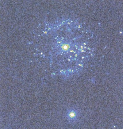 |
A nova can suddenly flares up in brilliance, by a factor of up to about one million, and then, over the next few months or years, fades back more or less to its original luminosity. It appears to be an event that occurs on the surface of a white dwarf in a close binary system when material flowing from the companion star onto the white dwarf's surface undergoes thermonuclear reactions, which trigger a violent explosion. The detonation blows surface material into space, leaving the underlying white dwarf unscathed. If the mass of the white dwarf is close to the Chandrasekhar limit of 1.4 Msun, hydrogen dragged from its companion burns to helium on its surface. The resulting increase in mass eventually triggers a Type Ia supernova explosion that completely destroys the white dwarf. Figure 08-12 is a recurrent nova in the constellation of Pyxis. It is surrounded by more than 2000 gaseous blobs packed into an area about 1 light year across. |
Figure 08-12 Nova [view |
large image] |
 |
 |
 |
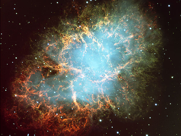
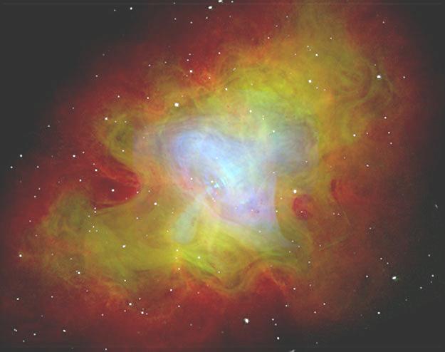
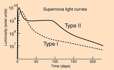
When stars with mass greater than 5 Msun exhaust their nuclear fuel, they collapse suddenly in a process called supernova explosion, which flings off huge amount of heavy elements into interstellar space. Super- novae can be classified into two types. Their characteristics are listed in Table 08-04 |
Figure 08-13 Crab Nebula, Visible Light [view large image] | Figure 08-14 Crab Nebula, Composite [view large image] | Figure 08-15 Crab Nebula, X-ray [view large image] |
below. Figures 08-13, 08-14, and 08-15 are images of the Crab Nebula taken at different wavelength. The Crab Nebula is a supernova remnant after an explosion at 1054 AD. |
| Characteristic | Type I | Type II |
|---|---|---|
| Initial Mass | < 8 Msun | 8 - 50 Msun |
| Light Curve | Smooth Decline | Decline + Plateau |
| Maximum Luminosity | 10 billion Lsun | ~ 1 billion Lsun |
| Mode of Energy Generation | Nuclear | Gravitational |
| Stellar Type | Old Population II | Young Population I |
| Hydrogen Absorption Lines | No | Yes |
| Binary System | Usually | No |
| Milky Way Frequency | ~ 1/36 year | ~ 1/44 year |
| Occurrence in Elliptical Galaxy | Yes | No |
 |
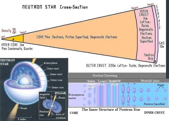 |
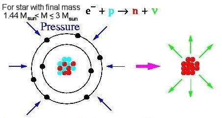
When the core of the star collapses to a density of about 1014 gm/cm3 (of the order of that in the nuclei) it causes the atomic electrons to combine with the nuclear protons in the electron capture reaction as shown in Figure 08-16. This is the point where gravitational forces have won out over the pressure supplied by nuclear matter. Figure 08-17 shows the structure of a neutron star in several layers over a depth of ~ 10 km: |
Figure 08-16 Electron Capture [view large image] |
Figure 08-17 Neutron Star, Structure [view large image] |
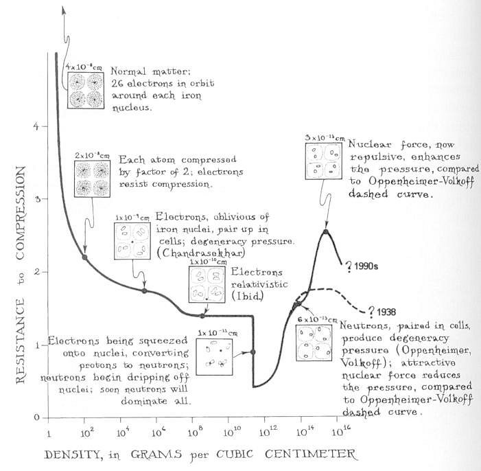 |
attached to the curve show what is happening to the microscopic matter as it is compressed from low densities to high. At normal densities, cold, dead matter is composed of iron. As the iron is squeezed from its normal density of 7.6 gm/cm3 up toward 100, then 1000 gm/cm3, the iron resists by the same means as a rock resists compression - the degeneracy-like motions of electrons. When the density has reached 100000 gm/cm3, the electron's degeneracy pressure completely overwhelm the electric forces with which the nuclei pull on the electrons. The electrons no longer congregate around the iron nuclei; they completely ignore the nuclei and form the electron gas moving around freely. At a density of about 107 gm/cm3 the motion of the electrons become relativistic (near the speed of light). |
Figure 08-18 Equation of State [view large image] |
 |
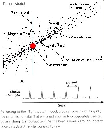 |
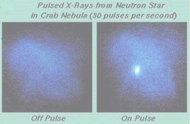
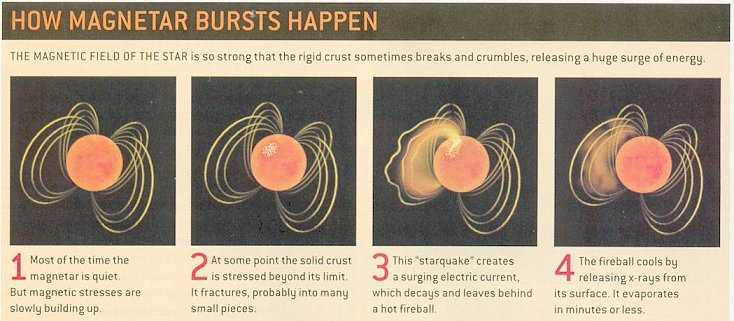
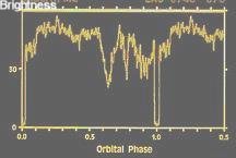
to 1.6x10⁻⁶ sec. Only a tiny, dense neutron star could spin this fast; larger stars (including white dwarfs) would be torn to shreds by centrifugal force. The magnetic field at the surface of a collapsing star grows in strength as the surface area of the star decreases (decreases in radius / increases in magnetic field strength ~ 1 / 105). The magnetic field strengths at the surfaces of neutron stars are likely to be between 108 and 1013 gauss. In some extreme examples (known as magnetars) they may be as high as 1015 gauss. Figure 08-19 shows the pulsar signal from the neutron star inside the Crab Nebula |
Figure 08-19 Pulsar Signal |
Figure 08-20 Pulsar Model [view large image] |
with a period of 0.03 sec in the X-ray range. |
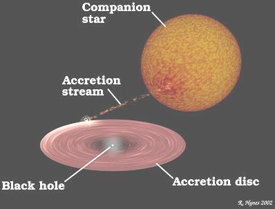 |
Most black holes are said to be stellar: formed from stars. It is estimated that the Milky Way contains 10 million of these black holes. Their mass can be 10 times that of the sun and the radius of event horizon can be a few kilometers. Because not even light can escape from inside the event horizon, it is hard to detect black holes. Astronomers get around this problem by indirect observations on some signatures, which are peculiar to a black hole. It usually involves the interaction of the black hole with its environment, e.g., a companion star. Figure 08-21 is a model of a stellar black hole drawing material (the accretion stream) from the companion star. The accretion stream forms an accretion disc before finally spiraling into the black hole and generates bursts of X-rays. |
Figure 08-21 Blackhole Model |
 |
 |
 |
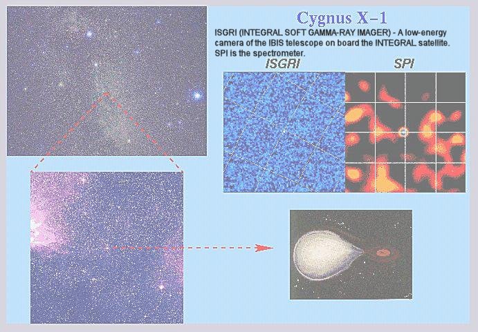
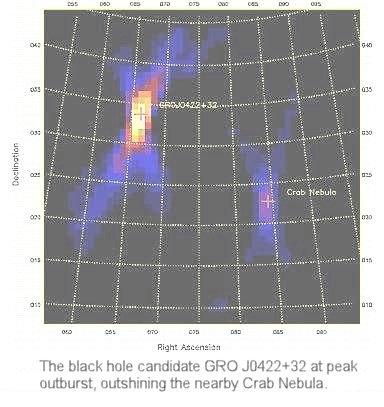
is probably the largest stellar black hole discovered; while the X-ray source GRO J0422+32 near V518 Persei seems to be the smallest with a mass of 3 to 5 Msun. |
Figure 08-22 Cygnus X-1 |
Figure 08-23 V404 Cyg |
Figure 08-24 GRS1915 [view large image] |
| Final Event | Initial Mass (Msun) / Type | Final Mass (Msun) | Life Time (109 yrs.) | Heaviest Element Synthesized | Residual Core |
|---|---|---|---|---|---|
| Gradual Cooling | < 0.1 / M7 | same | > 1000 | Helium | Brown Dwarf |
| Stellar Wind | < 0.4 / M5 | ~ same | > 200 | Helium | White Dwarf |
| Stellar Wind or Planetary Nebula |
< 1.0 / G2 | < 0.7 | > 10 | Helium or Carbon | White Dwarf |
| Planetary Nebula | < 3.0 / A0 | < 0.8 | > 0.35 | Oxygen | White Dwarf |
| Supernova, Type I / II | < 10 / B5 | < 1.5 | > 0.02 | Oxygen or Silicon | White Dwarf or Neutron Star |
| Supernova, Type II | < 15 / B1 | < 10 | > 0.01 | Silicon or Iron | Neutron Star or Black Hole |
| Supernova, Type II | < 30 / O8 | < 20 | > 0.004 | Iron | Black Hole |
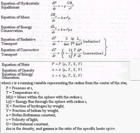 |
In most cases, the density, the temperature, and the chemical composition of a star change appreciably only over very long time intervals. For the Sun, only 1% of the hydrogen is depleted and converted into helium in one billion years . Thus the change induced by nuclear fuel depletion is entirely negligible. A static stellar model is appropriate for the Sun and most of the main sequence stars. Time does not appear in any equation under this circumstance. Whether it is static or dynamic, the stellar structure is governed by five basic equations. In mathematical terms, they are a set of inter-dependent differential equations (see Figure 08-25). A verbal description is given below for simulating the structure of a main sequence star. |
Figure 08-25 Stellar Model [view large image] |